Konstantin and I were honored with an ICML Outstanding paper award for our paper “Learning-Rate-Free Learning by D-Adaptation”. Besides the award, our implementation has already been downloaded nearly a million times over the last year (most before the award), and is seeing wide-spread use in training and fine-tuning deep learning models, particularly LoRAs.

Read on if you would like to know more about our work and the impact it is already having as a practical solution that removes the need to tune the baseline learning rate.

Adapting to D

Conference awards often elevate papers that take interesting new approaches to old problems, and this is certainly the case here. Our approach sounds like it wouldn’t work: we take an upper bound that would normally be used to show convergence, and we invert it, to instead give a lower bound $d_k$ on a key quantity $D=\parallel x_0-x_{\ast }\parallel$. Since $D$ plays the key role of the numerator of the step size in convex Lipscthiz optimization, we can use this bound $d_k$ to define a step-size:

$${\gamma }_k=\frac{d_k}{\sqrt{\sum _i^k{\parallel g_i\parallel }^2}}.$$

Using this step-size in a plug-and-play style gives the D-Adaptation method. Simple!

The particular bound we use is a slight refinement of existing convergence bounds:

$$\sum _{k=0}^n{d}_k\left(f\left(x_k\right)-f_{\ast }\right)\le D\parallel \sum _{k=0}^n{g}_k\parallel +\frac{1}{2}\sum _{k=0}^n{\gamma }_k{d}_k^2{\parallel g_k\parallel }^2-\frac{1}{2}{\gamma }_{n+1}{\parallel \sum _{k=0}^n{g}_k\parallel }^2,$$

and the rearrangement is simple. We first use that $f\left(x_k\right)-f_{\ast }\ge 0$, to give

$$0\le D\parallel \sum _{k=0}^n{g}_k\parallel +\frac{1}{2}\sum _{k=0}^n{\gamma }_k{d}_k^2{\parallel g_k\parallel }^2-\frac{1}{2}{\gamma }_{n+1}{\parallel \sum _{k=0}^n{g}_k\parallel }^2,$$

Then pull $D$ over to the left:

$$D\ge d_k=\frac{{\gamma }_{n+1}{\parallel \sum _{k=0}^n{g}_k\parallel }^2-\sum _{k=0}^n{\gamma }_k{d}_k^2{\parallel g_k\parallel }^2}{2\parallel \sum _{k=0}^n{g}_k\parallel }.$$

Why does this look crazy? Well for one thing, we have no reason to expect $d_k$ to be positive, in fact, it usually isn’t. The solution to the positivity issue turns out to be simple. Instead of using the bound directly, we define $d_k$ to be the max over the bounds over all previous steps. To “bootstrap” the process, we start with $d_0=10^{-8}$ or a similar small positive value. Given the seeming looseness of this approach, we wouldn’t expect this lower bound to provide a close estimate to $D$, but in fact it does! In practice, the $d$ sequence grows exponentially, from arbitrarily small initial $d_0$ to values as good as hand tuned choices. We are even able to show that in theory, it asymptotically approaches the true D to within a factor of 0.366.

Convergence properties

“Non-asymptotic results tell you ’what’s really going on’, but asymptotics tell you what’s *really* going on” - Sam Power

Our key theory result is simple: we show that for a sufficiently large number of training steps $n$, our approach yields convergence as fast as if you had of set the step size using knowledge of the true D from the beginning:

$$f\left({\widehat{x}}_n\right)-f\left(x_{\ast }\right)=\mathcal{}\left(\frac{\mathit{DG}}{\sqrt{n+1}}\right),$$

where ${\widehat{x}}_n$ is the average iterate, and $G$ is a bound on the gradient norms. This is an interesting result for a number of reasons. Firstly, it’s the first such “asymptotic” result for this problem class to have no additional log factors - you pay no penalty for not knowing D! Other methods for the problem class we consider: convex, non-smooth Lipschitz functions, require knowledge of other unknowns, such as $f\left(x_{\ast }\right)$ or require line searches, back-tracking or other complexities. A chief advantage of our method is it’s so damn simple.

The major down-side of this asymptotic result is that we don’t know how many optimization steps need to be taken, $n$, before this asymptotic behavior kicks in. Fortunately, in practice, it kicks in after less than a few hundred steps, typically 1-2% of the total training time at most. This corresponds to when the $d_k$ estimate becomes within a constant factor of the true $D$. We see this across more than 20 test problems, across deep-learning problems as well as simpler logistic regression problems.

The asymptotic bound we prove appears to be the true indictor of the behavior of our method in practice, although we give a non-asymptotic bound as well, which shows that the convergence is never worse than a log factor off the best-possible rate, even when $n$ is small. Approaches from the “parameter-free” literature such as coin-betting give slightly better non-asymptotic rates for this class (sqrt(log) factor difference), however we have developed an improved variant of D-Adaptation that matches the non-asymptotic rates of those parameter-free methods, known as Prodigy (https://arxiv.org/pdf/2306.06101.pdf). Prodigy seems to be an overall improvement over D-Adaptation in practice also, so we recommend its use as the primary variant of the method.

More on non-asymptotics

The non-asymptotic rate given by approaches such as coin betting for the average iterate is:

$$f\left({\widehat{x}}_n\right)-f\left(x_{\ast }\right)=\mathcal{}\left(\frac{\mathit{DG}\sqrt{\log <!--\; FUNCTION\; APPLICATION\; -->\left(1+D∕d_0\right)}}{\sqrt{n+1}}\right).$$

Essentially you pay a $\sqrt{\log <!--\; FUNCTION\; APPLICATION\; -->(1+D∕d_0)}$ penalty for not having knowledge of $D$ before-hand. There is a much simpler approach that gives essentially the same rate for this complexity class: Grid Search! In fact, the simple approach of running $R=\log <!--\; FUNCTION\; APPLICATION\; -->(D_{\max <!--\; FUNCTION\; APPLICATION\; -->}∕D_{\min <!--\; FUNCTION\; APPLICATION\; -->})$ runs with a log-spaced grid of D values (i.e. $10^{-8},10^{-7},10^{-6},\dots <!--\; FUNCTION\; APPLICATION\; -->$) bracketing the true D. Since our total step-budget is $n+1$, each run must be of length (n+1)/R, and so taking the best $\widehat{x}$ by function value gives a bound:

$$\begin{array}{llll}\hfill f\left({\widehat{x}}_n\right)-f\left(x_{\ast }\right)& =\mathcal{}\left(\frac{\mathit{DG}}{\sqrt{(n+1)∕R}}\right)& \hfill & \\ \hfill & =\mathcal{}\left(\frac{\mathit{DG}\sqrt{R}}{\sqrt{n+1}}\right)& \hfill & \\ \hfill & =\mathcal{}\left(\frac{\mathit{DG}\sqrt{\log <!--\; FUNCTION\; APPLICATION\; -->\left(D_{\max <!--\; FUNCTION\; APPLICATION\; -->}∕D_{\min <!--\; FUNCTION\; APPLICATION\; -->}\right)}}{\sqrt{n+1}}\right).& \hfill & \end{array}$$

Often in computer-science research we ignore log factors as unimportant, or “not-real”, but in this case, the log factor is very real! It corresponds to the cost of running multiple training runs and throwing away all but the best run.

Given this is the same sqrt(log) dependence as for coin betting, what differentiates parameter-free approaches such as coin-betting? They are developed for a much more general class of problems, Online Linear Optimization (OLO), and so when applied to convex non-smooth optimization as we do here, they are not able to make use of the additional problem structure. Note that the grid search method above obviously can’t achieve a sqrt-log-factor free rate asymptotically, since you have to actually perform each of the $R$ training runs. It’s unclear if coin-betting approaches can avoid the log factor asymptotically, this is an interesting direction for future research. Lower bounds are known for the online linear optimization setting that show that any non-asymptotic rate must include this sqrt-log factor.

Why previous parameter-free methods don’t work as well

A major component of our work was the effort it took to go from a theoretically nice algorithm to a practical method that works on deep learning problems. We had to identify why other learning-rate free methods fail, and we had to adapt our method to work on top of modern optimization methods such as Adam.

The key insight turned out to be SCHEDULING. By scheduling, I mean a sequence of constants that multiply the learning rate, that includes potentially warm-up at the beginning of training, and annealing of the learning rate towards the end of training.

Using theoretically motivated schedules such as $1∕\sqrt{k+1}$ learning rate decay turn out to work terribly in practice almost across the board on deep learning problems. Existing coin-betting approaches prior to our work all relied on very poorly performing schedules. This is why the COCOB method we tested as a baseline under-performed The schedule is an implicit part of the method, arising directly from the mathematical formulation, and so its difficult to apply an arbitrary schedule on top of it, in contrast, D-Adaptation natively supports the use of arbitrary schedules.

Using existing empirically motivated schedules, such as those already widely in use in deep learning practice, leads to huge improvements in performance. In collaboration with Ashok and Harsh, I have also been working on incorporating schedule support into practical parameter-free methods, giving a method we call Mechanic (https://arxiv.org/abs/2306.00144).

Practical performance of D-Adaptation

Our Adam variant of D-Adaptation is a drop-in replacement for the PyTorch Adam class, requiring no other changes to the code-base. We tested across a large selection of modern deep learning problems, including auto-regressive language models, image-classification, image-2-image tasks, object recognition, recommendation systems, masked-language models and more. In fact, we performed the largest comparison performed for any optimization paper for a new method, outside of 10+ author papers from Google.

D-Adaptation matched the final test performance of laboriously hand-tuned learning rates on 9 of 10 deep learning problems, and all 12 logistic regression problems tested. We have also received overwhelming feedback from the ML community that the method “just-works” and is a true viable replacement for hand-tuned learning rates.

ICML is not a theoretically focused venue; reviewers highly value papers whose contribution have clear practical impact together with strong theory. Before D-Adaptation, there were no methods that could be “dropped-in” to a code base without other changes to provide adaptivity to the learning rate that actually worked well in practice. The ease of use of our method and its clear practical utility were recognized by our reviewers, with final review scores of 9, 8 and 6. We were fortunate to have highly communicative reviewers, who suggested improvements, pointed out errors (even reviewing the appendix carefully!) and overall greatly improved our work. A triumph of peer review!

Limitations

D-Adapt Adam uses an additional memory buffer on top of regular Adam, and so it has overall higher memory use. It can also fail on problems where training is very unstable. We experienced issues with it’s convergence on ViT (vision transformer) training for example.

Since setting the learning rate globally with D-Adaptation requires aggregating dot products and norms from across all parameters, it will requiring syncing information across nodes when using sharded data-parallel training, which may have a performance hit. We found that applying it separately at the block or node level didn’t work well, the global syncing appears to be necessary.

Our theory also has limitations. It only applies in the deterministic setting, which is much more limited than the stochastic or online settings that other methods such as coin-betting or DoG have theory for. Given the method seems to work well for stochastic problems, I see developing theory for this case as an interesting research problem.

D-Adaptation MUST be used with a schedule. I have seen several comparisons against D-Adaptation that don’t mention the use of schedules, and likely omitted them. This is crucial for the performance of the method. We recommend the use of the linear decay schedule with potentially a warmup (5%?) if warmup is customary for the problem being tackled.

What’s Next

It’s rather annoying that we have to choose a schedule to use with D-Adaptation.... surely there is some way to determine data-adaptive schedules automatically? Stay tuned for a solution!

An introductory lecture on optimization for deep learning

A deep dive into momentum and the MADGRAD method

I've just open sourced an implementation of the MADGRAD optimizer that I developed together with Samy Jelassi. It out-performs Adam on every problem I've tried it on, and it has generalization performance comparable to SGD, avoiding the overfitting problems of adaptive methods entirely! Check it out here: https://github.com/facebookresearch/madgrad

I recently came across this remarkable randomized algorithm due to Seidel (1991) for linear programming in 2 dimensions that takes only time $O\left(n\right)$ for $n$ constraints (in expectation). It’s definitely worth a close inspection, so I thought I would write a short article about it.

Note that my presentation of this algorithm assumes that there are no redundant or colinear constraints, that the solution is bounded, and that the solution for each subproblem encountered is unique. These assumptions are easy to remove without slowing the algorithm down, but they complicate the presentation a little.

This algorithm is quite remarkable in its simplicity. It takes the form of an recursive algorithm, where we solve a base case, then add additional constraints 1 at a time. Every time we add a constraint, we consider if it changes the solution. It’s only when the old solution $v^{\prime }$ is outside the added constraint that we have to do any work, namely solving a simple 1D LP, which is trivially $O\left(m\right)$ time for $m$ constraints.

If we had to solve the 1D LP subproblem at every step the algorithm would have quadratic running time $({\sum }_{i=1}^{n}i=O\left(n^2\right)$). We avoid this because we pick the constraint $B$ to recurse on at each step randomly. Clearly we only have to solve that 1D LP if the randomly chosen constraint B forms part of the new solution to the problem (ignoring degenerate solutions), and since a solution is the intersection of 2 constraints, there is only a $2$ in $\left|H\right|$ chance that we randomly pick such a constraint.

It follows that the cost of each recursion in expectation is $\left|H\right|$ times $2∕\left|H\right|$ which is just 2, and we recurse $n$ times, giving us a $O\left(n\right)$ running time in expectation.

In the original presentation by Seidel, the algorithm is given in a general form, usable in higher dimensions as well. The difficulty is that the running time quickly gets out of hand as the dimension $d$ increases. The main obstacle is step 4 above, you essentially need to solve a $d-1$ dimensional LP, which is only slightly easier than your original LP in higher dimensions.

On a side note, there is an interesting discussion of this algorithm and related ones in the Wikipedia page for LP-type problems.

References

Seidel, Raimund (1991), "Small-dimensional linear programming and convex hulls made easy", Discrete and Computational Geometry, 6 (5): 423–434

(PDF version of this article is available)

The Bayes factor test is an interesting thing. Some Bayesians advocate it unequivalently, whereas others reject the notion of testing altogether, Bayesian or otherwise. This post takes a critical look at the Bayes factor, attempting to tease apart the ideas to get to the core of what it’s really doing. If you're used to frequentist tests and want to understand Bayes factors, this post is for you.

The Bayes factor test goes all the way back to Jeffreys’ early book on the Bayesian approach to statistics [Jeffreys, 1939]. Evidence for an alternative hypothesis $H_1$ against that of the null hypothesis $H_0$ is summarized by a quantity known as the Bayes factor. The Bayes factor is just the ratio of the data likelihoods, under both hypotheses and integrating out any nuisance parameters:

If this ratio is large, we can conclude that there is strong evidence for the alternative hypothesis. In contrast, if the inverse of this ratio is large, we have evidence supporting the null hypothesis. The definition of what is strong evidence is subjective, but usually a Bayes factor of 10 or more is considered sufficient.

The standard Bayes factor test against the point-null

Although Bayes factors are sometimes used for testing simple linear regression models against more complex ones, by far the most common test in practice is the analogue to the frequentist t-test, the Bayes factor t-test. Under the assumption of normality with unknown variance, it tests a null hypothesis of zero mean against non-zero mean.

This test is implemented in the BayesFactor R package with the ttestBF method. For the pairwise case it can be invoked with bf <- ttestBF(x = xdata, y=ydata). For a non-pairwise test just x can be passed in.

Statistical details of the test To apply the test we must formally define the two hypotheses in the form of statistical models. Jeffreys’ book is very pragmatic, and the modelling choices for this test reflect that. Since this is a t-test, we of course assume a normal distribution for the data for both hypothesis, so it just remains to just define the priors on it’s parameters in both cases.

We have essentially 3 parameters we have to place priors on: the mean $\mu$ of the alternative, the variance under the alternative ${\sigma }_1^2$ and the variance under the null ${\sigma }_0^2.$ The $\mu$ under the null is assumed to be $0$. We have to be extremely careful about the priors we place on these parameters. Reasonable seeming choices can lead to divergent integrals or non-sensical results very easily. We discuss this further below.

Variance Because the variance appears in both the numerator and denominator of the Bayes factor (the null and the alternative), we can use a “non-informative” improper prior of the form $p\left({\sigma }^2\right)=1∕{\sigma }^2$ for both. This prior causes the marginal likelihood integrals to go to infinity, but this cancels out between the numerator and denominator giving a finite value.

Mean The choice of a prior for the mean is a little more subjective. We can’t use an improper prior here, as the mean prior appears only in the numerator, and without the convenient cancelation with factors in the denominator, the Bayes factor won’t be well defined. Jeffreys argues for a Cauchy prior, which is just about the most vague prior you can use that still gives a convergent integral. The scale parameter of the Cauchy is just fixed to the standard deviation in his formulation. The BayesFactor package uses 0.707 times the standard deviation instead as the default, but this can be overridden.

What are the downsides compared to a frequentist $t$-test? The main downside is that the BF test is not as good by some frequentist measures than the tests that are designed to be as good as possible with respect to those measures. In particular, consider the standard measure of power at $\gamma$: the probability of picking up an effect of size $\gamma$ under repeated replications of the experiment. Depending on the effect size and the number of samples $n$, a Bayesian $t$-test often requires 2-4 times as much data to match the power of a frequentist $t$-test.

Implementation details The Bayes factor requires computing marginal likelihoods, which is a quite distinct problem from the usual posterior expectations we compute when performing Bayesian estimation instead of hypothesis testing. The marginal likelihood is just an integral over the parameter space, which can be computed using numerical integration when the parameter space is small. For this t-test example, the BayesFactor package uses Gaussian quadrature for the alternative hypothesis. The null hypothesis doesn’t require any integration since it consists of a single point.

Jefferys lived in the statistical era of tables and hand computation, so he derived several formulas that can be used to approximate the Bayes factor. The following formula in terms of the $t$-statistic $t=\bar{x}\sqrt{\left(n-1\right)∕s^2}$ works well for $n$ in the hundreds or thousands:

The sensitivity to priors

There are two types of priors that appear in the application of Bayes factors; The priors on the hypothesis $p\left(H_0\right)$, $p\left(H_1\right)$, and the priors on parameters that appears in marginal likelihoods, the $p\left({}_0|H_0\right),$ $p\left({}_1|H_1\right)$. Your prior belief ratio $p\left(H_1\right)∕p\left(H_0\right)$ is updated to form your posterior beliefs using the simple equation:

The ratio $p\left(H_1\right)∕p\left(H_0\right)$ is not formally considered part of the Bayes factor, but it plays an important role. It encodes your prior beliefs about the hypotheses. If you are using Bayes factors in a subjective fashion, to update your beliefs in a hypothesis after seeing data, then it is crucial to properly encode your prior belief in which hypothesis is more likely to be true. However, in practice everybody always takes this ratio to be $1$, following the ideals of objective Bayesian reasoning, where one strives to introduce as little prior knowledge as possible into the problem. If your writing a scientific paper, it’s reasonable to use 1 as anybody reading the paper can apply there own ratio as a correction to your Bayes factor, reflecting there own prior beliefs.

The prior ratio of the hypotheses plays an interesting part in the calibration of the Bayes factor test. One way of testing Bayes factors is to simulate data from the priors, and compare the empirical Bayes factors over many simulations with the true ratios. This involving sampling a hypothesis, $H_0$ or $H_1$, then sampling $$ then D. If the probability of sampling $H_0$ and $H_1$ is not equal at that first stage, then the observed Bayes factor will be off by the corresponding $p\left(H_1\right)∕p\left(H_0\right)$. This is somewhat of a tautology, as we are basically just numerically verifying the Bayes factor equation as written. Nevertheless, it shows that if the priors on the hypotheses don’t reflect reality, then the Bayes factor won’t either. Blind application of a Bayes factor test won’t automatically give you interpretable “beliefs”.

Parameter priors

The dependence of Bayes factors on the parameter priors $p\left({}_1|H_1\right)$ and $p\left({}_0|H_0\right)$ is really at the core of understanding Bayes factors. It is a far more concrete problem than the hypothesis likelihoods, as there is no clear “objective” choices we can make. Additionally, intuitions from Bayesian estimation problems do not carry over to hypothesis testing.

Consider the simple BF t-test given above. We described the test using the Cauchy prior on the location parameter of the Gaussian. Often in practice people use large vague Gaussian priors instead when doing Bayesian estimation (as opposed to hypothesis testing), as they tend to be more numerically stable than the Cauchy. However, it has been noted by several authors [Berger and Pericchi, 2001] that simply replacing the Cauchy with a wide Gaussian in the BF t-test causes serious problems. Suppose we use a standard deviation of $\nu$ in this wide prior ($\nu$ large). It turns out that Bayes factor scales asymptotically like:

where $t=\bar{x}\sqrt{\left(n-1\right)∕s^2}$ is the standard t-statistic of the data. The large $\nu$ that was chosen with the intent that it would be ’non-informative’ (i.e. minimally effect the result) turns out to directly divide the BF!

This is the opposite situation from estimation, where as $\nu$ increases is behaves more and more like the improper flat prior $p\left(\right)\propto 1$. We can’t use the flat prior in the BF t-test, but if we assume that the sample standard deviation $s$ matches the true standard deviation, we can perform a BF z-test instead. Using a flat prior on $$, we get a BF of:

Because the flat prior appears in the numerator only there is no clear scaling choice for it, so this expression is not in any sense calibrated (Several approaches to calibration appear in the literature, see Robert [1993]).

It is interesting to see what happens when we apply the Cauchy prior, as used in the standard form of the test. In that case we see approximate scaling like [Robert et al., 2009]:

A similar formula appears when the data standard deviation is assumed to be known also:

The $1+\frac{t^2}{n}$ part can also be written $1+\frac{\bar{x}}{s^2}$ in terms of the known standard deviation and the empirical mean, and clearly it is constant asymptotically; the expression on the whole scales similarly as in the unknown variance case.

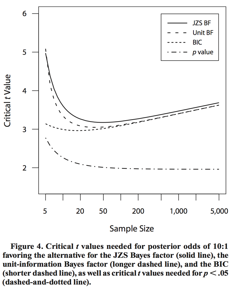
Lindley’s paradox

Lindley’s paradox refers to a remarkable difference in the behavior of Bayes factor tests compared to frequentist tests as the sample size increases. Under a frequentist t-test, we compute the $t$ statistic and compare it against a threshold that depends on $n$, and that decreases as $n$ increases, (Recall the definition of the $t$ statistic: $t=\bar{x}\sqrt{\left(n-1\right)∕s^2}$). In contrast the effective threshold used by the BF $t$-test actually increases as $n$ increases, although slowly, following roughly $\sqrt{logn}$. This difference is illustrated in the following plot lifted from Rouder et al. [2009]:

The effect of this difference is that for large sample sizes, a frequentist test can reject the null with small $p$ (say $p=0.05$), while a BF $t$-test run on the same data can strongly support the null hypothesis! As a concrete example, if we generate $n=50,000$ synthetic data points with mean $2∕\sqrt{50000}$, variance 1, then the BF $t$-test yields 0.028 for the alternative hypothesis (i.e. 36:1 odds for the null being true), whereas a frequentist $t$-test rejects the null with $p=0.0478$ (two-sided test).

It’s all well and good to argue the philosophical differences between Bayesian and frequentist approaches, but when they disagree so strongly, it becomes a practical issue. The key issue is the handling of small-effects. As $n$ increases and $s^2$ stays fixed, a fixed $t$ value of say 2 represents a smaller and smaller measured effect, namely:

Detecting small effects requires a large sample size, and the Bayesian $t$-test greatly prefers the null hypothesis over that of a small effect. This is usually described positively as a Occam’s razor effect, but it does have real consequences when we are attempting to find true small effects. Essentially, the BF test will require much more data pick up a small effect then a corresponding frequentist test. Often, this is viewed from the opposite side; that frequentist tests too easily reject the null hypothesis for large sample sizes. This is more of an issue when testing more complex models such as linear regressions with multiple coefficients. Unless the data was actually generated from a linear equation with Gaussian noise, large samples will inevitably reject simple null models. This is in contrast on simple point null hypothesis testing, where we can appeal to asymptotic normality.

Possible changes from the default Bayes factor test

Here we attempt to answer the following question: are the properties of the default Bayes factor test indicative of BF tests in general? As we see it, there are two main ways to modify the test: We can use a non-point hypothesis as the null, or we can change the alternative hypothesis in some fashion. We discuss these possibilities and their combination separately.

Changing the alternative hypothesis

The default Bayes factor t-test is formulated from a objectivist point of view: it’s designed so that the data can “speak for its self”, the priors used are essentially as vague as possible while still yielding a usable test. What about if we choose the prior for the alternative that gives the strongest evidence for the alternative instead? This obviously violates the likelihood principle as we choose the prior after seeing the data, but it is nevertheless instructive in that it indicates how large the difference between point NHST tests and BF tests are.

A reasonable class of priors to consider is those that are non-increasing in terms of $\left|\right|$ , as they have a single mode at $=0$. We discuss other priors below. Table 1 shows a comparison of p-values, likelihood ratios from the Neyman-Pearson likelihood ratio test, and a bound on BFs from any possible prior of this form. It is immediately obvious that according to this bound, any reasonable choice of prior yields much less evidence for the alternative then that suggested by the p-value. For example, the difference at p=0.001 is 18 fold, and the difference is larger for smaller $p$.

Although we disregarded multi-modal alternative priors above, they actually form an interesting class of tests. In terms of conservativeness, their BF is easily seen to be bounded by the likelihood ratio when using a prior concentrated on the maximum likelihood solution $\widehat{}$:

This ratio is simplify the Neyman-Pearson likelihood ratio for composite hypothesis, and it’s values are also shown in Table 1. This values are still more conservative than $p$-values by a factor of 2-5. Note that in a Neyman-Pearson test such as the frequentist $t$-test, this ratio is not read-off directly as an odds ratio as we are doing here; that’s why this NP odds ratio doesn’t agree directly with the p-value.

The interesting aspect of multi-modal priors is that they allow you to formulate a test that is more powerful for finding evidence of the null hypothesis. It can be shown that under the default BF t-test, evidence for the null accumulates very slowly when the null is true, where as evidence for the alternative accumulates exponentially fast when the alternative is true. Multi-modal priors can be formulated that fix this imbalance [Johnson and Rossell, 2010]. One simple case is a normal or Cauchy prior with a notch around the null $=0$ set to have low probability.

If we go a step further and consider the limits of sequences of improper priors, the Bayes factor can take essentially any value. Some particular “reasonable” sequences actually yield values very similar to $t$-test’s p-values [Robert, 1993] as their posterior probabilities, at least between 0.1 and 0.01. Their construction also places 0 probability mass in the neighborhood of the null point in the limit, so it is similar to the multi-modal priors discussed in the previous paragraph. Although this improper prior does actually avoid Lindley’s paradox, it is more of a theoretical construction; it is not recommend in practice, even by it’s discoverer [Robert, 1993].

Consequences for Lindley’s paradox

As discussed above, when restricting ourselves to well behaved proper priors, “Lindley’s paradox” as such can not be rectified by a careful choice of a proper prior on the alternative hypothesis. When one takes a step back and considers the consequences of this, Lindley’s paradox becomes much clearer, as a statement about objective priors rather than BF tests in general.

The central idea is this: It requires a lot of evidence to detect small effects when you use vague priors. The idea of running a long experiment when you use a vague prior is nonsensical from an experimental design point of view: large amounts of data are useful for picking up small effects, and if you expect such a small effect you should encode this sensibly in your prior. The default Cauchy prior used in the BF t-test essentially says that you expect a 50% chance that the absolute effect size (Cohen’s $d$) is larger than $1$, which is a completely implausible in many settings. For instance, if you are trying to optimize conversion rates on a website with say a 10% base conversion rate, an effect size of “1” is a 4x increase in sales! Some software defaults to 0.707 instead of 1 for the Cauchy scale parameter, but the effect is largely the same

Experimental design considerations are important in the choice of a prior, and the Bayesian justification of the Bayes factor depends on our priors being reasonable. The choice of using a particular BF test is not a full experimental design, just as for a frequentist it is not sufficient to just decide on particular test without regard to the eventual sample size. It is necessary to examine other properties of the test, so determine if it will behave reasonably in the experimental setting in which we will apply it. So in effect, Lindley’s paradox is just the statement that a poorly designed Bayesian experiment won’t agree with a less poorly designed frequentist experiment.

Put another way, if the Bayes factor is comparing two hypothesis, both of which are unlikely under the data, you won’t get reasonable results. You can’t identify this from examining the Bayes factor, you have to look at the experiment holistically. The extreme case of this is when neither hypothesis includes the true value of $$. In such cases, the BF will generally not converge to any particular value, and may show strong evidence in either direction.

An example

It is illustrative to discuss an example in the literature of this problem: a high profile case where the Bayesian and frequentist results are very different under a default prior, and more reasonable under a subjective prior. One such case is the study by Bem [2011] on precognition. The subject matter is controversial; Bem gives results for 9 experiments, in which 8 show evidence for the existence of precognition at the $p=0.05$ level! This obviously extraordinary claim lead to extensive examination of the results from the Bayesian view-point.

In Wagenmakers et al. [2011a], the raw data of Bem [2011] is analyzed using the default Bayesian t-test. They report Bayes factors towards the alternative (in decreasing order) of 5.88, 1.81, 1.63, 1.05, 0.88, 0.58, 0.47, 0.32, 0.29, 0.13 . So only one experiment showed reasonable evidence of precognition (5.88:1 for), and if you combine the results you get 19:1 odds against an effect.

In contrast, Bem et al. [2011] performed a Bayes factor analysis using informative priors on effect sizes, uses values considered reasonable under non-precognitive circumstances. The 3 largest Bayes factors for the existence of precognition they got were 10.1, 5.3 and 4.9, indicating substantial evidence!

The interesting thing here is that the vague prior used by Wagenmakers et al. [2011a] placed a large prior probability on implausibly large effect sizes. Even strong proponents of ESP don’t believe in such large effects, as they would have been easily detected in other past similar experiments. Somewhat counter-intuitively, this belief that ESP effects are strong if they exist at all yields a weaker posterior belief in the existence of ESP!

It should be noted that Wagenmakers et al. [2011b] responded to this criticism, but somewhat unsatisfactory in my opinion. Of course, even with the use of correct subjective Bayesian priors on the alternative hypothesis, these experiments are not sufficient to convince a skeptic (such as my self) of the existence of ESP! If one factors in the prior $p\left(H_1\right)∕p\left(H_0\right)$ and updates their beliefs correctly, you may go from a 1:1-million belief in ESP existing to a 1:76 belief (if you use the naive combined BF of 13,669 from Bem et al. [2011]).

Most reasonable people would consider the chance that a systematic unintentional error was made during the experiments to be greater than 1 in a thousand, and so not update their beliefs quite as severely. Regardless, several pre-registered replications of Bem’s experiments have failed to show any evidence of precognition [Ritchie et al., 2012].

Recommendations when using point-nulls

The general consensus in the literature is that single Bayes factors should not be reported. Instead the BFs corresponding to several different possible priors for the alternative hypothesis should be reported. Only if the conclusions are stable for a wide range of priors can they be reported as definitive. If the results are not stable, then it must be argued why a particular prior, chosen subjectively, is the best choice.

Bounds giving the largest or smallest possible Bayes factor over reasonable classes of priors, such as the bounds given in Berger and Jefferys [1991], can also be reported. The consideration of multiple possible priors is generally called “robust” Bayesian analysis.

Non-point nulls

As we showed above, under essentially any point-null Bayes factor t-test, the results are much more conservative than frequentist t-tests on the same data. But is this indicative of BF tests in general? It turns out Bayes factor tests that don’t use point-nulls behave much more like their frequentists counterparts [Casella and Berger, 1987].

But first, lets just point out that point-null hypotheses are fundamentally weird things. When we start assigning positive probability mass to single values, we move from the comfortable realm of simple distribution functions we can plot on a whiteboard, into the Terra pericolosa that is measure theory. As anybody who has done a measure theory course knows, common sense reasoning can easily go astray even on simple sounding problems. The “surprising” Occam’s razor effect seen in point-null BF tests is largely attributable to this effect. It can be argued that any prior that concentrates mass on a single point is not “impartial”, effectively favoring that point disproportionately [Casella and Berger, 1987].

One-sided tests

The simplest alternative to a point null test is a postive versus negative effect test, where the null is taken to be the entire negative (or positive) portion of the real line. This test is very similar in effect to a frequentist one sided test. Unlike the point-null case, both the alternative and null hypotheses spaces are the same dimension; in practice this means we can use the same unnormalized priors on both without running into issues. This test can be preformed using the BayesFactor R package with the ttestBF method, althought somewhat indirectly, by taking the ratio of two seperate point null tests:

Applying one-sided tests in the frequentist setting is routine (in fact often advocated [Cho and Abe, 2013]), it is surprising then that their theoretical properties are very different to two-sided tests. If we look at both Bayesian and frequentist approaches from the outside, using decision theory (with quadratic loss), we see a fundamental difference. For the one sided case, the Fisher p-value approach and obeys a weak kind of optimality known as admissibility [Hwang et al., 1992]: no approach strictly dominates it. In contrast, in the two-sided case neither the frequentist or the standard Bayesian approach is admissible, and neither dominates the other!

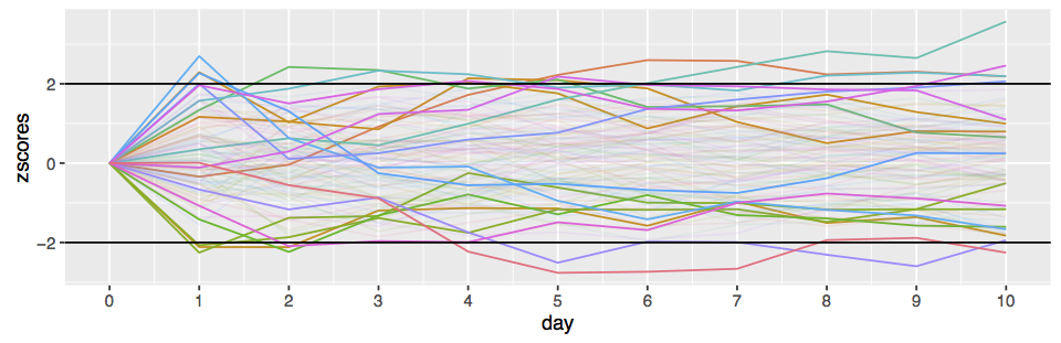
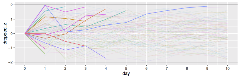
What does this tell us about sequential testing settings? The use of Bayes factor tests is sometimes advocated in the sequential testing setting, as their interpretation is not affected by early stopping. “Sequential testing” is when a test of some form of test is applied multiple times during the experiment, with the experiment potentially stopping early if the test indicates strong evidence of an effect. Using frequentist tests sequentially is problematic; the false-positive rate is amplified and special considerations must be made to account for this. See my previous post for details on how to perform the frequentist tests correctly.

The interpretation of the Bayes factor in contrast is unaffected by early stopping. Naive application of a point-null BF test does seem to perform reasonable in a sequential setting, as it’s naturally conservative nature results in few false positives being detected. However, as we pointed out above, one-sided non-point null tests are equally valid, and they are not particularly conservative. Just applying one sequentially gives you high false-positive rates comparable to the frequentist test. The false-positive rate is a frequentist property, and as such it is quite unrelated to the Bayesian interpretation of the posterior distribution.

Indeed, in most sequential A/B testing situations, such as website design tests, the one-sided non-point test seems the most reasonable, as the two hypothesis correspond more directly to the two courses of action that will be taken after the test concludes: Switch all customers to design A or design B.

So, should I use a point null hypothesis?

Here we start to move outside the realm of mathematics and start to meander into the realm of philosophy. You have to consider the purpose of your hypothesis test. Point-nulls enforce a strong Occam’s razor effect, and depending on the purpose of your test, this may or may not be appropriate.

The examples and motivation used for null hypothesis testing in the original formulation of the problem by Jeffreys came from physics. In physics problems testing for absolute truth is a much clearer proposition. Either an exotic particle exists or it doesn’t, there is no in-between. This is far cry from the psychology, marketing and economics problems that are more commonly dealt with today, where we always expect some sort of effect, although potentially small and possibly in the opposite direction from what we guessed apriori.

You need a real belief in the possibility of zero effect in order to justify a point null test. This is a real problem in practice. In contrast, by using non-point null tests you will be in closer agreement with frequentist results, and you will need less data to make conclusions, so there is a lot of advantages to avoiding point null tests.

It is interesting to contrast modern statistical practice in high energy physics (HEP) with that of other areas where statistics is applied. It is common practice to seek “five sigma” of evidence before making a claim of a discovery in HEP fields. In contrast to the usual $p\le 0.05$ requirements, the difference is vast. Five sigma corresponds to about a 1-in-1million $p$ value. However, if you view the five sigma approach as a heuristic approximation to the point-null BF test, the results are much more comparable. The equivalent $t$ statistic needed for rejection of the point null under the Bayesian test scales with the amount of data. HEP experiments often average over millions of data points, and it is in that multiple-million region where the rejection threshold, when rephrased in terms of the $t$ statistic, is roughly five.

Concluding guidelines for applying Bayes factor tests

• Don’t use point-null Bayesian tests unless the point null hypothesis is physically plausible.
• Always perform a proper experimental design, including the consideration of frequentist implications of your Bayesian test.
• Try to use an informative prior if you are using a point null test; non-informative priors are both controversial and extremely conservative. Ideally show the results under multiple reasonable priors.
• Don’t blindly apply the Bayes factor test in sequential testing situations. You need to use decision theory.

References

It’s amazing the amount of confusion on how to run a simple A/B test seen on the internet. The crux of the matter is this: If you're going to look at the results of your experiment as it runs, you can not just repeatedly apply a 5% significance level t-test. Doing so WILL lead to false-positive rates way above 5%, usually on the order of 17-30%.

Most discussions of A/B testing do recognize this problem, however the solutions they suggest are simply wrong. I discuss a few of these misguided approaches below. It turns out that easy to use, practical solutions have been worked out by clinical statistician decades ago, in papers with many thousands of citations. They call the setting “Group Sequential designs” [Bartroff et al., 2013]. At the bottom of this post I give tables and references so you can use group sequential designs in your own experiments.

What's wrong with just testing as you go?

The key problem is this: Whenever you look at the data (whether you run a formal statistical test or just eyeball it) you are making a decision about the effectiveness of the intervention. If the results look positive and you may decide to stop the experiment, particularly if it looks like the intervention is giving very bad results.

Say you make a p=0.05 statistical test at each step. On the very first step you have a 5% chance of a false positive (i.e. the intervention had no effect but it looks like it did). On each subsequent test, you have a non-zero additional probability of picking up a false positive. It’s obviously not an additional 5% each time as the test statistics are highly correlated, but it turns out that the false positives accumulate very rapidly. Looking at the results each day for a 10 day experiment with say 1000 data points per day will give you about an accumulated 17% false positive rate (According to a simple numerical simulation) if you stop the experiment on the first p<0.05 result you see.

---

---

---

---

The error-spending technique

They key idea of “Group Sequential” testing is that under the usual assumption that our test statistic is normally distributed, it is possible to compute the false-positive probabilities at each stage exactly using dynamic programming. Since we can compute these probabilities, we can also adjust the test’s false-positive chance at every step so that the total false-positive rate is below the threshold $\alpha$ we want. This is know as the error spending approach. Say we want to run the test daily for a 30 day experiment. We provide a 30 element sequence ${\alpha }_i$ of per step error chances, which sums to less than say $\alpha =0.05$. Using dynamic programming, we can then determine a sequence of thresholds, one per day, that we can use with the standard z-score test. The big advantage of this approach is that is a natural extension of the usual frequentist testing paradigm.

The error spending approach has a lot of flexibility, as the error chances can be distributed arbitrarily between the days. Several standard allocations are commonly used in the research literature.

Of course, libraries are available for computing these boundaries in several languages. Tables for the most common settings are also available. I’ve duplicated a few of these tables below for ease of reference.

Recommended approach

1. Choose a $\alpha$-spending function, from those discussed below. The Pocock approach is the simplest.
2. Fix the maximum length of your experiment, and the number of times you wish to run the statistical test. I.e. daily for a 30 day experiment.
3. Lookup on the tables below, or calculate using the ldbounds or GroupSeq R packages, the $z$-score thresholds for each of the tests you will run. For example, for the Pocock approach, $\alpha =0.01$, 10 tests max, use $z=3.117$ for every test. For the O’brien-Fleming approach it will be the sequence $\left\{8,5.82,4.95,4.29,3.8,3.46,3.19,2.98,2.80,2.66\right\}.$
4. Start the experiment.
5. For each test during the course of experiment, compute the $z$-score to the threshold, and optionally stop the test if the score exceeds the threshold given in the lookup table.

Real valued example

The simplest case of A/B testing is when each observation for each user is a numerical value, such as a count of activity that day, the sales total, or some other usage statistic. In this case the $z$-score when we have $n_a$ data points from group $a$ and $n_b$ from group $b$ with means and standard deviations $\mu$ and $\sigma$ is:

For the $k$th trial, just compare the $z$ value here to the $k$th threshold from the appropriate table below, if it exceeds it you may stop the experiment.

Conversions example

If in our A/B test we are testing if the click through rate or purchase chance improves, we use a slightly different formula. Let $p$ be the click through proportions and $n$ the total views (i.e. $n_a{p}_a=$conversions in group $A$). Then

As above, for the $k$th trial, just compare the $z$value here to the $k$th row of the appropriate table below, if it exceeds it you may stop the experiment.

Assumptions

• We are assuming the distribution of test statistic is normally distributed, with known variance. If you did STATS101, you are probably ok with this assumption, but those of you who did STATS102 are no doubt objecting. Shouldn’t you be using a t-test or chi-square test? What about the exact binomial test for conversions? The fact is that unless you are getting only a tiny amount of data between tests, you just don’t need to worry about this. If you are getting tiny amounts of data, you can’t hope to pick up any difference between the A/B groups over short time scales. Just run your test less regularly!
  The effect sizes we hope to see in A/B testing are much smaller than those in other areas of statistics such as clinical trials, so we usually can’t expect to get statistical significance in the small data regime where the normality approximation brakes down.
• Fixed maximum experiment length. This is an annoying problem. Often we would like to just keep running the experiment until we get some sort of effect. The difficulty is that we have to spread the chance of false-positives across the duration of the experiment. We could potentially use a error-spending function that drops off rapidly, so that the total error probability is summable. However, I would not recommend this. Instead, do a power calculation to determine the length of the experiment needed to pick up the minimum effect size that you would care about in practice. Then you can use that length for the experiment.
  In practice you will always see some sort of effect/uplift if you run a long enough experiment. There is no real world situation where the A/B groups behave exactly the same.
• Equally distributed tests. We are assuming above that we have the exact same amount of data gathered between tests. Fortunately this assumption is not too crucial to the correctness of the test. It is actually quite easy to correct for differing intervals using the R software discussed. Say you are in the common situation where you see much less data over the weekend than for a weekday. The ldbounds R package lets you calculate the sequence of $z$-score boundaries for variable intervals. you just feed in the time between tests as a normalized sequence that sums to $1$. For example, for a 7 day experiment starting on Monday, where the expected volume of data is half on Saturday and Sunday, you would just use something like:
  
  b <- bounds(cumsum(c(rep(1/6, 5), 1/12, 1/12)), iuse=c(1, 1), alpha=c(0.025, 0.025)) 
  print(b$upper.bounds) 
  [1] 5.366558 3.710552 2.969718 2.538649 2.252156 2.178169 2.088238

  The iuse argument controls the $\alpha$ spending function used (here we used the O’Brien-Fleming approach) and alpha gives the false-positive rate on either side (we are doing a $0.05$ fpr two-sided test here).

• Two-sided tests. The approach described above is that of a two-sided test. I allow for the effect of the intervention to be both potentially positive and negative. This is obviously more conservative then assuming it can only be positive, but I think in practice you should always use two-sided tests for A/B experiments. It’s hard to justify the assumption that the intervention can’t possibly have a negative effect!
• Why should I use this approach when Wald’s SPRT test is optimal? Wald’s theory of sequential testing is based around testing a single point hypothesis against another point hypothesis. While this approach is nearly as good as is possible for the simple point-point case, there is no clear generalization to the case of testing a point hypothesis of zero effect against the “composite” hypothesis of non-zero effect. In Wald’s 1945 book, several approaches are suggested, but they have known deficiencies [Sec 5.2 Tartakovsky et al., 2013]. Lordon’s 2-SPRT [Lordon, 1976] is the modern SPRT variant that is most commonly used. It requires setting an indifference region around 0 instead of a fixing the measurement points in advance, so the experimental design decisions are a little different. I intend to write more about the 2-SPRT in the future.

Bayesian approaches

Some people attempt to perform Bayesian tests by putting a prior on their data and computing “credible intervals” (or equivalently posterior probabilities) instead of confidence intervals. The classical “likelihood principle” states that Bayesian statistical quantities do not change under sequential testing, however under the Bayesian methodology estimation is fundamentally different from hypothesis testing, and trying to convert interval estimates to tests doesn’t work. The intuition is fairly simple: If Bayesian tests are immune to the sequential testing problem but Frequentist tests are not, then techniques like credible intervals which agree with frequentist confidence intervals on simple problems can’t then be used for Bayesian tests.

In general the best approach is to combine the Bayesian estimates with decision theory. This involves assigning a cost to each datapoint gathered, as well as determining the cost due to the test coming to the wrong solution.

I’m a strong proponent of Bayesian statistics, but I find it next to impossible in practice to determine these two costs. The frequentist approach of controlling false-positive rates is much easy to apply in a business context. The main exception is for per-user personalization or advert placement where the business decisions have to be made automatically. In that case the techniques studied for multi-arm Bandits or contextual bandits are natural automatic applications of the decision theory approach. They are far outside the scope of this post however.

The other Bayesian approach

The most commonly suggested Bayesian approach is the Bayes Factor (BF) test, a potential drop in replacement for frequentist tests. Indeed, A. Wald (the progenitor of sequential testing) way back in his 1945 book suggests a similar approach to a BF test [Sec. 4.1.3, Wald, 1945].

Unfortunately the bayes factor test often gives counter-intuitive and sometimes radically different results from frequentist tests. This is known as Lindley’s paradox [Lindley, 1957]. This doesn’t invalidate BF results, but you do need to fully understand the implications to use them in practice. I intend to write a another post going into detail about bayes factor tests, and their pitfalls and advantages over frequentist approaches.

Interactive tool

The GroupSeq R package provides a very easy to use GUI for calculating the stopping boundaries for most of the above settings. It can also do power calculations and stopping intervals. I’ve put a few screenshots of it in action below.

Power calculations

Powe calculations are typically used with frequentist experiments to determine the length of the experiment required to pick up effects of a certain magnitude. Power calculations can still be done for group sequential tests, using the R tools mentioned above. Like with the $z$-score boundary calculations, multiple integrals need to be evaluated numerically, so it is somewhat of a black-box.

Power calculations can also be used to select from the various error spending approaches above. Just run the power calculation for each approach, then choose the one that gives the smallest required experiment length.

Pocock 1977 tables (for two sided tests)

Pocock’s approach uses the exact same $z$-score threshold at every test. Values for larger $N$ (the total number of tests) or irregularly spaced test intervals may be calculated using the GroupSeq R package. The test $\alpha$ values here illustrated how much more conservative you need to be. For example, when running 10 tests during the experiment, you effectively have to run a $z$-test at the $\alpha =0.01$ level to get an effective $0.05$ false positive rate.

O’brien-Fleming style tables (for two sided tests)

This approach is essentially the most natural generalization of Wald’s SPRT test to the group-sequential case with composite hypothesis. This test is much less likely to stop at the early stages of the test than the other approaches, but more likely to stop in the later tests. Instead of reporting the tables from their paper I give the stopping boundaries for a version of their approach [O’brien and Fleming, 1979] adapted to the error-spending algorithm implemented in the ldbounds library.

In the computation below we cap the $z$-score stopping boundaries at $8$, as this is the default for the ldbounds library.

References

A colleague of mine has recently released a deep learning library for Haskell called Grenade. Probably the most interesting aspect is the use of dependent typing and other sophisticated functional programming tricks which are not normally seen in machine learning libraries. At the moment the library is in the proof of concept stage. You can basically use any combination of convolutional and fully connected layers, but training is single threaded using BLAS.

I've went through the hundreds of ICML 2016 papers and curated a subset that look interesting to me. In no particular order:

---

I've ported the NIPS 2016 template so that it can be used within LyX. You can download the template here: https://github.com/adefazio/nips-lyx-template. Only minimal changes were needed to the default LyX settings. I had to change the encoding and font settings to match the NIPS style since LyX's values conflicted with the preamble. If you have any issues with it, let me know.

This post describes the newly developed class of variance reduction techniques in stochastic optimisation, which are fast and simple alternatives to the traditional stochastic gradient descent (SGD) method. I give a light introduction here, focused on actually applying the methods in practice.

But first: Ye Old SGD

Quite possibly the most important algorithm in machine learning, SGD is simply a method for optimizing objective functions that consist of a sum or average of terms:

The SGD method maintains an estimate $x_k$ of the solution at step $k$, and at each step:

At it’s most basic, this update is just an approximation of the classical gradient descent technique, where we take the non-random step $x_{k+1}=x_k-\gamma f^{\prime }\left(x_k\right).$ The step size parameter $\gamma$ here is just a constant, which depending on the problem may need to be adjusted down at each step. Variance reduction methods build upon SGD by modifying the core update in various ways.

SAGA

The SAGA method is a simple modification of SGD, where we remember the last gradient evaluated for each datapoint, and use this to correct the SGD step to reduce its variance. These past gradients are stored in a table. We denote the previous gradient for datapoint j as $f_j^{\prime }\left({\varphi }_j^k\right)$. The core step is as follows:

Source code for SAGA and the accelerated variant point-saga is available on github. Some points about the algorithm:

• Storing the past gradients is typically fast and low cost. For logistic regression or least squares, it reduces to storing a single real value per datapoint instead of a full gradient. Similar reductions apply to neural networks. When the storage cost is high, the SVRG method described below can be used instead.
• The table average $\frac{1}{n}{\sum }_{i=1}^n{f}_i^{\prime }\left({\varphi }_i^k\right)$ is of course cached rather then recalculated at each step.
• Notice that there is only really two extra terms on top of the usual SGD step. The two terms also trivially cancel when you take the expectation with respect to $j$. So the expected step direction is a gradient step, just like with SGD.
• The step above assumes you already have a table of gradients. If you are just starting the algorithm, do the first pass over the data in-order (instead of random), and use the table average over only the data seen so far in the step. Alternatively, just do regular SGD steps during the first pass.
• The requirement for randomly sampling datapoints instead of doing in-order passes turns out to be absolutely crucial for it to work.
• Implementing the step efficiently when the gradients are sparse is a little subtle, but possible. See the SAGA paper for details and example code.
• SAGA supports non-differentiable regularisers through the use of proximal operators. See the paper for details.

Why variance reduction methods?

VR methods like SAGA have entirely different convergence properties than SGD. On strongly convex problems they are able to converge linearly ($O(log\left(1∕k\right)$), instead of the much slower $O\left(1∕k\right)$ convergence possible with the SGD method (which requires careful iterate averaging). Linear convergence on a stochastic method is quite remarkable, up until recently no such methods were known. It’s also fast linear convergence, compared to the theoretical rate for regular gradient descent, it makes 1/3 the progress each step, but each step is only a single datapoint evaluation rather than a full batch gradient. For large datasets that can be millions of times faster. A schematic illustration of the practical speedup is below, labeled as "incremental gradient":

Other variance reduction techniques

SAGA is perhaps the most straightforward of the variance reduction techniques. The other VR methods have advantages in certain situtations, there is no clear best method in all cases. We list the main methods here, each has several variants as well:

SAG

is the earliest of these VR methods developed. It doesn’t actually take the gradient direction in expectation, rather it introduces a small bias with the potential for a lower variance in the gradient estimate. Unfortunately SAG is hard to extend from the point of view of the theory.

SVRG

is the direct predecessor of SAGA that makes a different trade-off. It avoids storing gradients, but at the expense of computing two gradients per step instead of one. It also has a more complex double loop formulation, where the outer loop requires a recalculation of the full-data gradient. In most cases the extra computation makes it slower than SAGA, but it does have some applications.

Finito/Miso

take a step derived indirectly from the dual formulation of the problem, while avoiding any dual computation. They don’t work efficently on sparse problems, but are perhaps the fastest methods on dense problems.

SDCA

is a purely dual method. It can be applied to some non-differentiable problems unlike the other methods here, but it is complex to apply efficently to other problems such as logistic regression. It also has the nice properly of avoiding tunable parameters on problems with L2 regularisation. For practical application it crucially requires a non-degenerate amount of strong convexity though.

References

Daryl J. Bem. Feeling the future: Experimental evidence for anomalous retroactive influences on cognition and affect. Journal of Personality and Social Psychology, 2011.
Daryl J. Bem, Jessica Utts, and Wesley O. Johnson. Must psychologists change the way they analyze their data? a response to wagenmakers, wetzels, borsboom, & van der maas. 2011.
James O. Berger and William H. Jefferys. The application of robust bayesian analysis to hypothesis testing and occam’s razor. Technical report, Purdue University, 1991.
James O. Berger and Luis R. Pericchi. Objective bayesian methods for model selection: Introduction and comparison. IMS Lecture Notes - Monograph Series, 2001.
J.O. Berger and R.L. Wolpert. The Likelihood Principle. Institute of Mathematical Statistics. Lecture notes : monographs series. Institute of Mathematical Statistics, 1988. ISBN 9780940600133. URL https://books.google.com.au/books?id=7fz8JGLmWbgC.
George Casella and Roger L. Berger. Reconciling bayesian and frequentist evidence in the one-sided testing problem. Journal of the American Statistical Association, 82(397):106–111, 1987. ISSN 0162-1459. doi: 10.1080/01621459.1987.10478396.
Hyun-Chul Cho and Shuzo Abe. Is two-tailed testing for directional research hypotheses tests legitimate? Journal of Business Research, 66(9):1261 – 1266, 2013. ISSN 0148-2963. doi: http://dx.doi.org/10.1016/j.jbusres.2012.02. 023. URL http://www.sciencedirect.com/science/article/pii/S0148296312000550. Advancing Research Methods in Marketing.
Jiunn Tzon Hwang, George Casella, Christian Robert, Martin T. Wells, and Roger H. Farrell. Estimation of accuracy in testing. Ann. Statist., 20(1):490–509, 03 1992. doi: 10.1214/aos/1176348534. URL http://dx.doi.org/10.1214/aos/1176348534.
Harold Jeffreys. Theory of Probability. 1939.
V. E. Johnson and D. Rossell. On the use of non-local prior desities in bayesian hypothesis tests. Journal of the Royal Statistical Society, 2010.
Stuart J. Ritchie, Richard Wiseman, and Christopher C. French. Failing the future: Three unsuccessful attempts to replicate bem’s ‘retroactive facilitation of recall’ effect. PLoS ONE, 2012.
Christian P. Robert. A note on jeffreys-lindley paradox. Statistica Sinica, 1993.
Christian P. Robert, Nicolas Chopin, and Judith Rousseau. Harold jeffreys’s theory of probability revisited. Statistical Science, 2009.
Jeffrey N. Rouder, Paul l. Speckman, Dongchu Sun, Richard D. Morey, and Geoffrey Iverson. Bayesian t tests for accepting and rejecting the null hypothesis. Psychonomic Bulletin & Review, 2009.
Eric Jan Wagenmakers, Ruud Wetzels, Denny Borsboom, and Han van der Maas. Why psychologists must change the way they analyze their data: The case of psi. Journal of Personality and Social Psychology, 2011a.
Eric Jan Wagenmakers, Ruud Wetzels, Denny Borsboom, and Han van der Maas. Why psychologists must change the way they analyze their data: The case of psi: Clarifications for bem, utts, and johnson (2011). Journal of Personality and Social Psychology, 2011b.
How to do A/B testing with early stopping correctly
Jay Bartroff, Tze Leung Lai, and Mei-Chiung Shih. Sequential Experimentation in Clinical Trials. Springer, 2013.
D. V. Lindley. A statistical paradox. Biometrika, 44:187–192, 1957.
Gary Lordon. 2-sprt’s and the modified kiefer-weiss problem of minimizing an expected sample size. The Annals of Statistics, 4:281–291, 1976.
Peter C. O’brien and Thomas R. Fleming. A multiple testing procedure for clinical trials. Biometrics, 35, 1979.
Stuart J. Pocock. Group sequential methods in the design and analysis of clinical trials. Biometrika, 64, 1977.
Alexander Tartakovsky, Igor Nikiforov, and Michéle Basseville. Sequential Analysis: Hypothesis Testing and Changepoint Detection. CRC Press, 2013.
A. Wald. Sequential tests of statistical hypotheses. Ann. Math. Statist., 16(2):117–186, 06 1945. doi: 10.1214/aoms/1177731118. URL http://dx.doi.org/10.1214/aoms/1177731118.
Machine Learning in Haskell!