It’s amazing the amount of confusion on how to run a simple A/B test seen on the internet. The crux of the matter is this: If you're going to look at the results of your experiment as it runs, you can not just repeatedly apply a 5% significance level t-test. Doing so WILL lead to false-positive rates way above 5%, usually on the order of 17-30%.
Most discussions of A/B testing do recognize this problem, however the solutions they suggest are simply wrong. I discuss a few of these misguided approaches below. It turns out that easy to use, practical solutions have been worked out by clinical statistician decades ago, in papers with many thousands of citations. They call the setting “Group Sequential designs” [Bartroff et al., 2013]. At the bottom of this post I give tables and references so you can use group sequential designs in your own experiments.
What's wrong with just testing as you go?
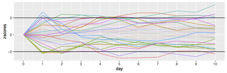
The key problem is this: Whenever you look at the data (whether you run a formal statistical test or just eyeball it) you are making a decision about the effectiveness of the intervention. If the results look positive and you may decide to stop the experiment, particularly if it looks like the intervention is giving very bad results.
Say you make a p=0.05 statistical test at each step. On the very first step you have a 5% chance of a false positive (i.e. the intervention had no effect but it looks like it did). On each subsequent test, you have a non-zero additional probability of picking up a false positive. It’s obviously not an additional 5% each time as the test statistics are highly correlated, but it turns out that the false positives accumulate very rapidly. Looking at the results each day for a 10 day experiment with say 1000 data points per day will give you about an accumulated 17% false positive rate (According to a simple numerical simulation) if you stop the experiment on the first p<0.05 result you see.
The error-spending technique
They key idea of “Group Sequential” testing is that under the usual assumption that our test statistic is normally distributed, it is possible to compute the false-positive probabilities at each stage exactly using dynamic programming. Since we can compute these probabilities, we can also adjust the test’s false-positive chance at every step so that the total false-positive rate is below the threshold we want. This is know as the error spending approach. Say we want to run the test daily for a 30 day experiment. We provide a 30 element sequence of per step error chances, which sums to less than say . Using dynamic programming, we can then determine a sequence of thresholds, one per day, that we can use with the standard z-score test. The big advantage of this approach is that is a natural extension of the usual frequentist testing paradigm.
The error spending approach has a lot of flexibility, as the error chances can be distributed arbitrarily between the days. Several standard allocations are commonly used in the research literature.
Of course, libraries are available for computing these boundaries in several languages. Tables for the most common settings are also available. I’ve duplicated a few of these tables below for ease of reference.
Recommended approach
- Choose a -spending function, from those discussed below. The Pocock approach is the simplest.
- Fix the maximum length of your experiment, and the number of times you wish to run the statistical test. I.e. daily for a 30 day experiment.
- Lookup on the tables below, or calculate using the ldbounds or GroupSeq R packages, the -score thresholds for each of the tests you will run. For example, for the Pocock approach, , 10 tests max, use for every test. For the O’brien-Fleming approach it will be the sequence
- Start the experiment.
- For each test during the course of experiment, compute the -score to the threshold, and optionally stop the test if the score exceeds the threshold given in the lookup table.
Real valued example
The simplest case of A/B testing is when each observation for each user is a numerical value, such as a count of activity that day, the sales total, or some other usage statistic. In this case the -score when we have data points from group and from group with means and standard deviations and is:
For the th trial, just compare the value here to the th threshold from the appropriate table below, if it exceeds it you may stop the experiment.
Conversions example
If in our A/B test we are testing if the click through rate or purchase chance improves, we use a slightly different formula. Let be the click through proportions and the total views (i.e. conversions in group ). Then
As above, for the th trial, just compare the value here to the th row of the appropriate table below, if it exceeds it you may stop the experiment.
Assumptions
- We are assuming the distribution of test statistic is normally distributed, with known variance. If you
did STATS101, you are probably ok with this assumption, but those of you who did STATS102 are no
doubt objecting. Shouldn’t you be using a t-test or chi-square test? What about the exact binomial test for
conversions? The fact is that unless you are getting only a tiny amount of data between tests, you just don’t
need to worry about this. If you are getting tiny amounts of data, you can’t hope to pick up any difference
between the A/B groups over short time scales. Just run your test less regularly!
The effect sizes we hope to see in A/B testing are much smaller than those in other areas of statistics such as clinical trials, so we usually can’t expect to get statistical significance in the small data regime where the normality approximation brakes down. - Fixed maximum experiment length. This is an annoying problem. Often we would like to just keep running the
experiment until we get some sort of effect. The difficulty is that we have to spread the chance of false-positives
across the duration of the experiment. We could potentially use a error-spending function that drops off
rapidly, so that the total error probability is summable. However, I would not recommend this. Instead, do a
power calculation to determine the length of the experiment needed to pick up the minimum effect size that
you would care about in practice. Then you can use that length for the experiment.
In practice you will always see some sort of effect/uplift if you run a long enough experiment. There is no real world situation where the A/B groups behave exactly the same. - Equally distributed tests. We are assuming above that we have the exact same amount of data gathered between tests.
Fortunately this assumption is not too crucial to the correctness of the test. It is actually quite easy to correct for
differing intervals using the R software discussed. Say you are in the common situation where you see much less
data over the weekend than for a weekday. The ldbounds R package lets you calculate the sequence of
-score
boundaries for variable intervals. you just feed in the time between tests as a normalized sequence that sums to
.
For example, for a 7 day experiment starting on Monday, where the expected volume of data is half on Saturday and
Sunday, you would just use something like:
b <- bounds(cumsum(c(rep(1/6, 5), 1/12, 1/12)), iuse=c(1, 1), alpha=c(0.025, 0.025))
print(b$upper.bounds)
[1] 5.366558 3.710552 2.969718 2.538649 2.252156 2.178169 2.088238The iuse argument controls the spending function used (here we used the O’Brien-Fleming approach) and alpha gives the false-positive rate on either side (we are doing a fpr two-sided test here).
- Two-sided tests. The approach described above is that of a two-sided test. I allow for the effect of the intervention to be both potentially positive and negative. This is obviously more conservative then assuming it can only be positive, but I think in practice you should always use two-sided tests for A/B experiments. It’s hard to justify the assumption that the intervention can’t possibly have a negative effect!
- Why should I use this approach when Wald’s SPRT test is optimal? Wald’s theory of sequential testing is based around testing a single point hypothesis against another point hypothesis. While this approach is nearly as good as is possible for the simple point-point case, there is no clear generalization to the case of testing a point hypothesis of zero effect against the “composite” hypothesis of non-zero effect. In Wald’s 1945 book, several approaches are suggested, but they have known deficiencies [Sec 5.2 Tartakovsky et al., 2013]. Lordon’s 2-SPRT [Lordon, 1976] is the modern SPRT variant that is most commonly used. It requires setting an indifference region around 0 instead of a fixing the measurement points in advance, so the experimental design decisions are a little different. I intend to write more about the 2-SPRT in the future.
Bayesian approaches
Some people attempt to perform Bayesian tests by putting a prior on their data and computing “credible intervals” (or equivalently posterior probabilities) instead of confidence intervals. The classical “likelihood principle” states that Bayesian statistical quantities do not change under sequential testing, however under the Bayesian methodology estimation is fundamentally different from hypothesis testing, and trying to convert interval estimates to tests doesn’t work. The intuition is fairly simple: If Bayesian tests are immune to the sequential testing problem but Frequentist tests are not, then techniques like credible intervals which agree with frequentist confidence intervals on simple problems can’t then be used for Bayesian tests.
In general the best approach is to combine the Bayesian estimates with decision theory. This involves assigning a cost to each datapoint gathered, as well as determining the cost due to the test coming to the wrong solution.
I’m a strong proponent of Bayesian statistics, but I find it next to impossible in practice to determine these two costs. The frequentist approach of controlling false-positive rates is much easy to apply in a business context. The main exception is for per-user personalization or advert placement where the business decisions have to be made automatically. In that case the techniques studied for multi-arm Bandits or contextual bandits are natural automatic applications of the decision theory approach. They are far outside the scope of this post however.
The other Bayesian approach
The most commonly suggested Bayesian approach is the Bayes Factor (BF) test, a potential drop in replacement for frequentist tests. Indeed, A. Wald (the progenitor of sequential testing) way back in his 1945 book suggests a similar approach to a BF test [Sec. 4.1.3, Wald, 1945].
Unfortunately the bayes factor test often gives counter-intuitive and sometimes radically different results from frequentist tests. This is known as Lindley’s paradox [Lindley, 1957]. This doesn’t invalidate BF results, but you do need to fully understand the implications to use them in practice. I intend to write a another post going into detail about bayes factor tests, and their pitfalls and advantages over frequentist approaches.
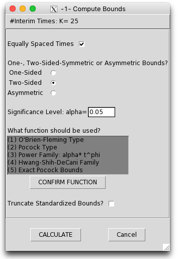
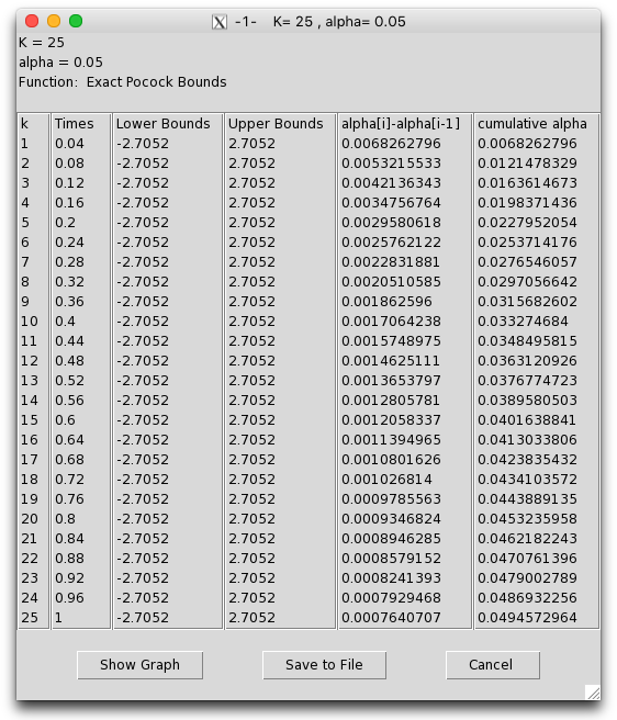
Interactive tool
The GroupSeq R package provides a very easy to use GUI for calculating the stopping boundaries for most of the above settings. It can also do power calculations and stopping intervals. I’ve put a few screenshots of it in action below.
Power calculations
Powe calculations are typically used with frequentist experiments to determine the length of the experiment required to pick up effects of a certain magnitude. Power calculations can still be done for group sequential tests, using the R tools mentioned above. Like with the -score boundary calculations, multiple integrals need to be evaluated numerically, so it is somewhat of a black-box.
Power calculations can also be used to select from the various error spending approaches above. Just run the power calculation for each approach, then choose the one that gives the smallest required experiment length.
Pocock 1977 tables (for two sided tests)
Pocock’s approach uses the exact same -score threshold at every test. Values for larger (the total number of tests) or irregularly spaced test intervals may be calculated using the GroupSeq R package. The test values here illustrated how much more conservative you need to be. For example, when running 10 tests during the experiment, you effectively have to run a -test at the level to get an effective false positive rate.
| For | For | |||
| test | -score | test | -score | |
| 1 | 0.05 | 1.960 | 0.01 | 2.576 |
| 2 | 0.0294 | 2.178 | 0.0056 | 2.772 |
| 3 | 0.0221 | 2.289 | 0.0041 | 2.873 |
| 4 | 0.0182 | 2.361 | 0.0033 | 2.939 |
| 5 | 0.0158 | 2.413 | 0.0028 | 2.986 |
| 6 | 0.0142 | 2.453 | 0.0025 | 3.023 |
| 8 | 0.0120 | 2.512 | 0.0021 | 3.078 |
| 10 | 0.0106 | 2.555 | 0.0018 | 3.117 |
| 12 | 0.0097 | 2.585 | 0.0016 | 3.147 |
| 15 | 0.0086 | 2.626 | 0.0015 | 3.182 |
| 20 | 0.0075 | 2.672 | 0.0013 | 3.224 |
O’brien-Fleming style tables (for two sided tests)
This approach is essentially the most natural generalization of Wald’s SPRT test to the group-sequential case with composite hypothesis. This test is much less likely to stop at the early stages of the test than the other approaches, but more likely to stop in the later tests. Instead of reporting the tables from their paper I give the stopping boundaries for a version of their approach [O’brien and Fleming, 1979] adapted to the error-spending algorithm implemented in the ldbounds library.
In the computation below we cap the -score stopping boundaries at , as this is the default for the ldbounds library.
|
z-scores (two-sided tests) |
||
| 1.00 | 0.05 |
1.96 |
| 1.00 | 0.01 |
2.576 |
| 2.00 | 0.05 |
2.963,1.969 |
| 2.00 | 0.01 |
3.801,2.578 |
| 3.00 | 0.05 |
3.710,2.511,1.993 |
| 3.00 | 0.01 |
4.723,3.246,2.589 |
| 4.00 | 0.05 |
4.333,2.963,2.359,2.014 |
| 4.00 | 0.01 |
5.493,3.802,3.044,2.603 |
| 5.00 | 0.05 |
4.877,3.357,2.680,2.290,2.031 |
| 5.00 | 0.01 |
6.168,4.286,3.444,2.947,2.615 |
| 6.00 | 0.05 |
5.367,3.711,2.970,2.539,2.252,2.045 |
| 6.00 | 0.01 |
6.776,4.740,3.803,3.257,2.892,2.626 |
| 8.00 | 0.05 |
6.232,4.331,3.481,2.980,2.644,2.401,2.215,2.066 |
| 8.00 | 0.01 |
8.000,8.000,4.442,3.807,3.381,3.071,2.833,2.643 |
| 10.00 | 0.05 |
6.991,4.899,3.930,3.367,2.989,2.715,2.504,2.336,2.197,2.081 |
| 10.00 | 0.01 |
8.000,8.000,5.071,4.289,3.812,3.463,3.195,2.981,2.804,2.656 |
| 15.00 | 0.05 |
8.000,8.000,4.900,4.189,3.722,3.382,3.120,2.910,2.738,2.593, 2.469,2.361,2.266,2.182,2.107 |
| 15.00 | 0.01 |
8.000,8.000,8.000,8.000,4.731,4.295,3.964,3.699,3.481,3.297, 3.139,3.002,2.881,2.774,2.678 |
| 20.00 | 0.05 |
8.000,8.000,8.000,4.916,4.337,3.942,3.638,3.394,3.193,3.024, 2.880,2.754,2.643,2.545,2.457,2.378,2.305,2.239,2.179,2.123 |
| 20.00 | 0.01 |
8.000,8.000,8.000,8.000,8.000,5.076,4.615,4.302,4.050,3.837, 3.653,3.494,3.353,3.229,3.117,3.016,2.925,2.841,2.764,2.693 |
| 25.00 | 0.05 |
8.000,8.000,8.000,8.000,4.919,4.436,4.093,3.820,3.594,3.404, 3.241,3.100,2.975,2.865,2.766,2.676,2.595,2.521,2.452,2.389, 2.331,2.277,2.226,2.179,2.134 |
| 25.00 | 0.01 |
8.000,8.000,8.000,8.000,8.000,8.000,5.517,4.878,4.565,4.315, 4.107,3.928,3.769,3.629,3.504,3.390,3.287,3.193,3.107,3.027, 2.953,2.884,2.820,2.760,2.703 |
| 30.00 | 0.05 |
8.000,8.000,8.000,8.000,8.000,4.933,4.505,4.204,3.956,3.748, 3.568,3.413,3.276,3.154,3.045,2.946,2.857,2.775,2.700,2.631, 2.566,2.506,2.451,2.398,2.349,2.303,2.260,2.219,2.180,2.143 |
| 30.00 | 0.01 |
8.000,8.000,8.000,8.000,8.000,8.000,8.000,8.000,4.986,4.731, 4.510,4.318,4.144,3.991,3.853,3.728,3.615,3.512,3.416,3.329, 3.247,3.172,3.101,3.035,2.973,2.914,2.859,2.807,2.758,2.711 |
| 50.00 | 0.05 |
8.000,8.000,8.000,8.000,8.000,8.000,8.000,8.000,5.185,4.919, 4.669,4.454,4.279,4.118,3.976,3.848,3.731,3.625,3.526,3.436, 3.352,3.274,3.201,3.132,3.068,3.008,2.951,2.898,2.847,2.798, 2.752,2.709,2.667,2.627,2.589,2.552,2.517,2.484,2.452,2.421, 2.391,2.362,2.334,2.307,2.281,2.256,2.232,2.208,2.186,2.164 |
| 50.00 | 0.01 |
8.000,8.000,8.000,8.000,8.000,8.000,8.000,8.000,8.000,8.000, 8.000,8.000,8.000,8.000,5.173,4.938,4.739,4.589,4.452,4.339, 4.230,4.133,4.040,3.954,3.874,3.797,3.726,3.658,3.594,3.533, 3.475,3.419,3.367,3.316,3.268,3.222,3.178,3.135,3.095,3.055, 3.018,2.981,2.946,2.912,2.880,2.848,2.817,2.788,2.759,2.731 |
| 60.00 | 0.05 |
8.000,8.000,8.000,8.000,8.000,8.000,8.000,8.000,8.000,8.000, 5.292,4.977,4.718,4.525,4.372,4.229,4.101,3.984,3.876,3.776, 3.684,3.598,3.518,3.443,3.373,3.307,3.244,3.185,3.129,3.076, 3.025,2.977,2.932,2.888,2.846,2.806,2.767,2.730,2.695,2.661, 2.628,2.596,2.566,2.536,2.508,2.480,2.453,2.427,2.402,2.378, 2.355,2.332,2.309,2.288,2.267,2.246,2.227,2.207,2.188,2.170 |
| 60.00 | 0.01 |
8.000,8.000,8.000,8.000,8.000,8.000,8.000,8.000,8.000,8.000, 8.000,8.000,8.000,8.000,8.000,8.000,8.000,5.036,4.902,4.778, 4.662,4.539,4.439,4.345,4.258,4.170,4.092,4.019,3.947,3.880, 3.817,3.756,3.698,3.643,3.590,3.539,3.491,3.444,3.399,3.356, 3.315,3.275,3.236,3.199,3.163,3.128,3.095,3.062,3.030,3.000, 2.970,2.941,2.913,2.886,2.859,2.834,2.808,2.784,2.760,2.737 |
References
Jay Bartroff, Tze Leung Lai, and Mei-Chiung Shih. Sequential Experimentation in Clinical Trials. Springer, 2013.
D. V. Lindley. A statistical paradox. Biometrika, 44:187–192, 1957.
Gary Lordon. 2-sprt’s and the modified kiefer-weiss problem of minimizing an expected sample size. The Annals of Statistics, 4:281–291, 1976.
Peter C. O’brien and Thomas R. Fleming. A multiple testing procedure for clinical trials. Biometrics, 35, 1979.
Stuart J. Pocock. Group sequential methods in the design and analysis of clinical trials. Biometrika, 64, 1977.
Alexander Tartakovsky, Igor Nikiforov, and Michéle Basseville. Sequential Analysis: Hypothesis Testing and Changepoint Detection. CRC Press, 2013.
A. Wald. Sequential tests of statistical hypotheses. Ann. Math. Statist., 16(2):117–186, 06 1945. doi: 10.1214/aoms/1177731118. URL http://dx.doi.org/10.1214/aoms/1177731118.
What if we are running an AB test with several segments, and we look at its results multiple times?
We have to apply a Bonferroni correction for the >2 number of segments, and to this correction too.
Are the two corrections independent? How should I change the sigma-threshold in this case?
Did you ever figure this out?
Hey Aaron,
Strange that it is only now that I find your post! You make some very good points on both the practical application of the frequentist approaches, as well as your critique for some of the Bayesian ones. I actually go deeper in my critique – on more fundamental grounds, but thumbs up for that!
I’m sure you’d be interested to read a white paper I’ve recently written “Efficient A/B Testing in Conversion Rate Optimization: The AGILE Statistical Method (free download at https://www.analytics-toolkit.com/whitepapers.php?paper=efficient-ab-testing-in-cro-agile-statistical-method ). In it I use a more advanced version of some of the procedures you propose, including adding futility stopping (power-spending functions) to the mix. These significantly improve the efficiency gains from using AGILE, which run from 20% to 80%, depending on the relation between the true theta and the design theta for the alternative hypothesis for which power calculation is done.
Do let me know what you think about it!
Best,
Georgi